Multi-Linear Regression

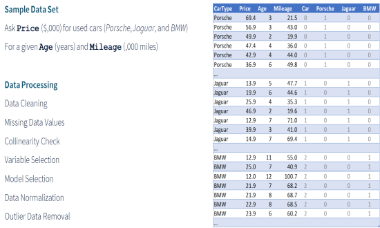
Overview

Data Processing techniques, which deal with the collection, cleaning, and analysis of data, have been in manual use for decades. With recent developments in machine learning techniques, many statistical algorithms are today used for semi-automatic data processing.

This page talks about different dimensions of data processing and the automation support provided by data processing languages like R.

To illustrate different dimensions of data processing, we have used the Three Cars sample data set, that gives the market Price of Porsche, Jaguar, and BMW used cars for their given Age and Mileage.

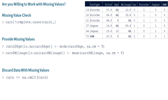
Missing Data Values

Missing Data are a common problem for data analysis. This is especially true when the available data set is created through manual data entry; e.g. in a call center. While missing data may not be an issue with some data analysis and machine learning models, some others may give wrong results with missing data.

R language provides the complete.cases() function, which can be used to identify records that have missing data. Depending on the statistical model(s) being used for data analysis, you can decide what actions you would like to take to handle the missing data.

In some cases, you may want to completely delete records with missing data. While in other cases, you may want to provide the missing data using simple mean, interpolation, or other statistical functions.

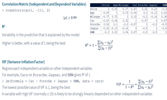
Collinearity Check

Multicollinearity refers to a scenario where there is a strong linear relationship between two or more independent variables. This is an issue, especially with linear regression models.

For example, in a multivariate linear regression, if two input variables x₁ and x₂ define an output variable y = α • x₁ + β • x₂, where there is a strong linear relationship between x₁ and x₂, then it would not be possible to accurately find the values of α and β that define the impacts of input variables x₁ and x₂ on the output variable y. In our example, the variable Car holds perfect multicollinearity with variables Porsche, Jaguar, and BMW, as the lm() function gives R² of 1.

Simply dropping the redundant input variables solves the problem.

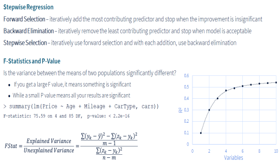
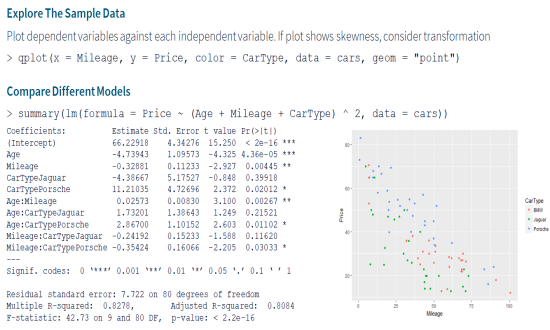
Variable Selection

Dimensionality Reduction is an important aspect of data processing, which helps in reducing the complexity of data analysis by selecting a subset of independent variables that best explain the variance in the dependent variable(s). For many real-life use-cases, the data set contains large number of independent variables, many of which are redundant and do not contribute in building a reliable prediction model.

Many different step-wise regression techniques are used to select the best subset of independent variables. For example, forward selection, backward elimination, step-wise selection, etc. F-test and p-value are commonly used statistical tests for comparing the models at different regression steps.

Model Selection

Model Selection deals with selecting a statistical model that best represents a given data set. In the most simple form a dependent variable may hold linear relationships with one or more independent variables. For example, for our use-case we can present in R the relationship of Price ~ Age + Mileage + CarType. The lm() function then finds the estimates for Price = α + β • Age + γ • Mileage + δ • CarType. However, you may want to also try a non-linear relationship of the dependent variable with independent variables. In our use-case, we tried a model with first level interactions between independent variables; represented in R as Price ~ (Age + Mileage + CarType) ^ 2. As you can see in the image, interaction of Age:Mileage is quite significant.

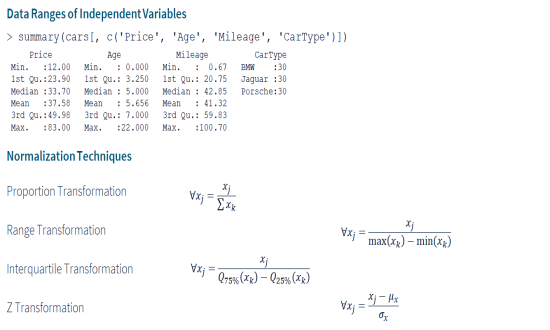
Data Normalization

Normalization of data is an important step in data processing, especially when there is an order of magnitude difference in the values of different independent variables. In a more complex scenario, you may want to standardize the data set if it is a coalition of multiple data sets from different sources. For example, employee performance ratings by different managers in an organization.

There are different techniques available for normalization. A simple approach could be range transformation, where you divide the data with its range. If the data is normally distributed, you can use z-transformation to convert it to standard normal distribution.

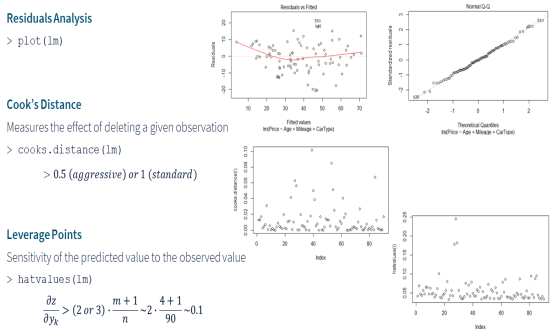
Outlier Data Removal

Outlier detection deals with identification and removal of suspicious data points that significantly differ from the normal trends in the data set. In most cases, these are due to errors in observation or recording. The outliers create a skew and may cause serious problems in the data analysis.

Cook’s distance is a common technique to find the impact of a data point on the regression analysis. Values with high Cook’s distance are good candidates for a closer examination.

Leverage point analysis is another common technique to find the sensitivity of the predicted values to the observed values. Points with high deviation are possible anomalies in the data set.