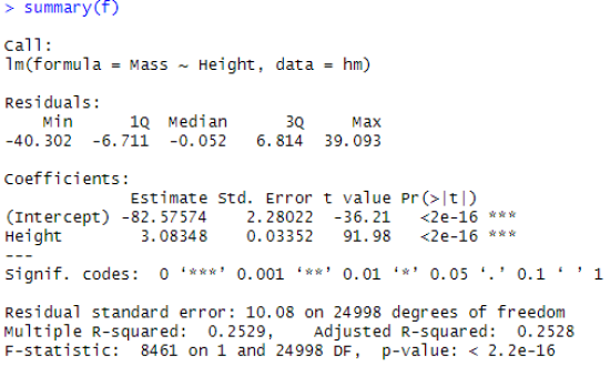
Linear Modeling in R

Linear Model Coefficients

Summary of the linear model in R gives the following coefficient details:

• Estimate for the (Intercept) is the expected value of response variable when predictor variables are zero. The Height estimate here is the rate at which we expect the Mass to change with height. In our example, the Mass changes at a rate of 3.08348 lb/inch. It is always good to spot check the intercept number to make sure it seems reasonable – in our example it does not.
• Std. Error is the expected difference in our estimate if we ran the model on similar data sets. As a rule of thumb, the value should be an order of magnitude less than the coefficient estimate.
• t value is Estimate ÷ Std. Error. It is a measure of how many standard deviations our coefficient estimate is away from the mean (zero) in a standard normal distribution. We want it to be far away from zero as this would indicate that there is a relationship between Height and Mass.
• Pr(^lt;|t|), also called p-value, is the probability that the variable is not relevant. In our example, 2e-16 means that the odds that the variable is meaningless is about 1/5e+15.
• Stars represent significance level of the variable, based on the p-value. *** for high significance and * for low significance. Blank is bad, Dots are okay, Star is good, and More Stars are very good.

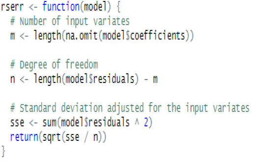
Residual Standard Error

The residuals are the difference between the actual values of the response you’re predicting and predicted values from your regression.

The Residual Standard Error is simply the standard deviation of your residuals.

The Degrees of Freedom is the difference between the number of observations included in your training sample and the number of variables used in your model, including the intercept.

For our data set, rserr function returns 10.07952, which matches the summary above.

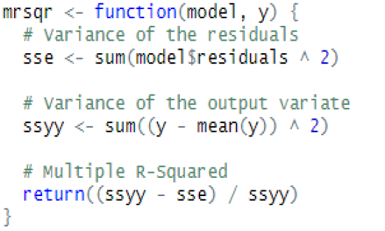
Multiple R Squared

Multiple R² (or simply R²) is the metric for evaluating the goodness of fitness of your model. Higher is better with 1 being the best.

The value corresponds to the amount of variability in the prediction that is explained by the model.

WARNING: While a high R-squared indicates good correlation, correlation does not always imply causation.

For our data set, mrsqr function returns 0.2528667, which matches the summary above.

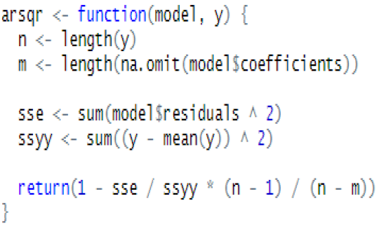
Adjusted R Squared

Adjusted R² (or R_adj²) can be interpreted as a less biased estimator of the goodness of fitness of your model, when compared to R². This takes into account the sudden increase in the value of R² when extra predictor variables are added to the model.

The R_adj² can be negative and its value will always be less than or equal to that of R². If we introduce predictor variables in the model one at a time, in the order of their importance, we will observe that R_adj² will reach a maximum, before it starts decreasing. The model for which R_adj² is maximum has the ideal combination of predictor variables, without any redundant terms.

For our data set, arsqr function returns 0.2528368, which matches the summary above.

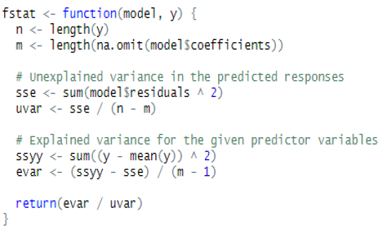
F Statistic

F-Statistic performs an F-test on the model. This takes the parameters of our model and compares them to a model that has fewer parameters.

In theory the model with more parameters should fit better.

• If the model with more parameters (your model) does not perform significantly better than a model that has fewer parameters, the F-test will have a high p-value (probability that there is NOT a significant boost).
• If the model with more parameters (your model) is better than a model that has fewer parameters, you will have a lower p-value.

The DF, or degrees of freedom, pertains to the number of predictor variables in the model.

For our data set, fstat function returns 8460.554, which matches the summary above.